ストレンジネス3次元核図表
スクリプトとデータシートを作成しました。
見た目やデータは簡単に書き換えられると思うのでLicenseの範囲でご自由にお使いください。
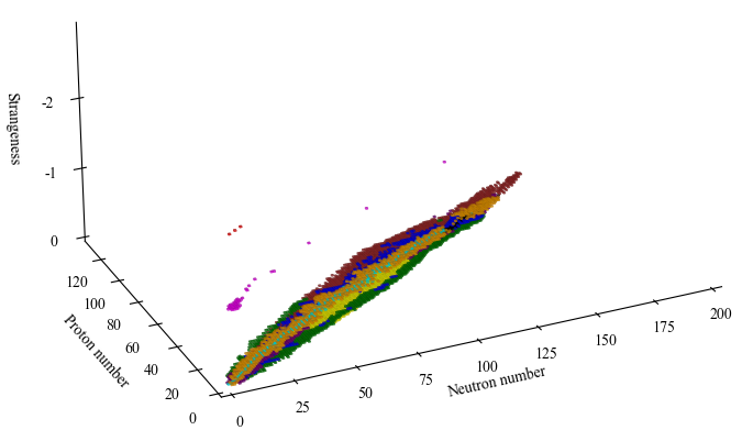
参考にしたのは以下の3つのサイトや実装
マインツ大のハイパー核データチャート
東北大金田さんのHP (アイデア)
本来の3次元核図表はストレンジネスではなくこんなやつ
(onsanai氏のツイートより)
ざっくり pic.twitter.com/Gmc5jTMhIK
— onsa (@onsanai) 2024年7月22日
Windows PCをUbuntuにする際の注意 (Secure Boot設定)
備忘録
企業から購入したWindows11インストール済みPCのOSをUbuntu22.04に変更し、機械学習用の環境構築を進めていたところ...
nvidia-diriverの変更時に突然ターミナルがピンク色になってパニックに。
UEFI BIOSのSecure Boot設定が有効になっているためドライバの変更時にキー認証等を求められるようでした。
再起動してUEFI BIOSのAdvanced MenuからBootの設定画面へ
Secure Bootを "UEFI Windows OS" -> "Other OS"に変更。
その後、環境構築を最初からやり直したら警告灯が出ることなく、うまくいきました。
VS Code + Docker + GPUサーバーによる開発環境の設定 (Tiny ImageNetを題材に)
目的
学生ゼミの課題を題材にVS Codeを用いたサーバーへのログインDockerでの作業手順のチュートリアルを作成する。
Tiny imagenetについてはスタンフォード大の以下のページを参照してください。
cs231n.stanford.edu

Tiny ImageNet using PyTorch. I joined in FreeCodeCamp course where… | by Lokesh Para | Medium
セットアップ、実行の手順を示します。
間違いや非推奨なものがあればコメント等でぜひご指摘・指導ください。
以下の記載ルール&注意事項
- $で始まるのはターミナル(シェル)に打ち込むコマンド。コピぺするときは$の後ろからコピーしてください。
- 今回実行した環境のCUDAは諸事情でバージョンが古いためdocker imageやコードのバージョンも古くなっています。
- ご指摘があった場合、記載内容・推奨方法を変更することがあります。
GPUマシンに接続
$ ssh hogehoge
$ cd # <作業するdirectoryに移動>
CUDA Versionの確認
$ nvidia-smi

+-----------------------------------------------------------------------------+
| NVIDIA-SMI 440.33.01    Driver Version: 440.33.01    CUDA Version: 10.2     |
|-------------------------------+----------------------+----------------------+
| GPU  Name        Persistence-M| Bus-Id        Disp.A | Volatile Uncorr. ECC |
| Fan  Temp  Perf  Pwr:Usage/Cap|         Memory-Usage | GPU-Util  Compute M. |
|===============================+======================+======================|
|   0  ************...  On   | 00000000:18:00.0 Off |                  N/A |
| 27%   24C    P8    13W / 250W |      0MiB / 11019MiB |      0%      Default |
+-------------------------------+----------------------+----------------------+
docker imageをpull(ダウンロード)
このマシンでは"CUDA Version: 10.2"とあるので対応するdocker imageを以下のサイトから探す。
tecsingularity.com
$ docker pull tensorflow/tensorflow:2.1.0-gpu-py3
以下のコマンドを実行してpullしたimageが表示されればok
$ docker images
REPOSITORY                     TAG                 IMAGE ID            CREATED             SIZE
tensorflow/tensorflow          2.1.0-gpu-py3       e2a4af785bdb        3 years ago         4.11GB
docker containerの生成
dockerfileを作成する。以下のリポジトリにDockerfileやコードをいくつか置いてみました。
$ git clone https://github.com/ayumisalt/tiny_imagenet_tutorial.git
$ cd tiny_imagenet/docker
4つのファイルがこのディレクトリに存在しています。
- Dockerfile : build時に実行するコマンドがまとまっている。
- requirements_apt.txt: apt-getで取得するコマンドを入れたリスト
- requirements_pip.txt: pip install で取得するパッケージのリスト
- zshrc: おすすめのzshrcの設定
zshrcはこちらのサイトから拝借
少し凝った zshrc · GitHub
Dockerfileの中身をlessコマンドなどで眺めてみるとrequirements_*.txtやzshrcが読み込まれている部分を確認できると思います。
必要があればrequirements_*.txtに自分が作業に使いたいパッケージを入れてください。
docker buildコマンドでimageを生成
docker build . -t <作成するimageの名前>
docker runコマンドでコンテナを作成
$ docker run --name <コンテナの名前> --gpus all -it --ulimit memlock=-1 --ulimit stack=67108864 -v <作業dirがあるdisk (例:data00)> --workdir=<作業dirのpath> --ipc=host <先ほど作成したimageの名前> /usr/bin/zsh
上記コマンドにて、コンテナ内で使用するGPUについては以下のように記載します。
gpuが使用できることを確認する。
コンテナ内でpythonをインタープリターモードで起動し、次のコマンドを実行。
>>> from tensorflow.python.client import device_lib
>>> device_lib.list_local_devices()
以下のような出力が得られればok
$ python
Python 3.6.9 (default, Nov  7 2019, 10:44:02)
[GCC 8.3.0] on linux
Type "help", "copyright", "credits" or "license" for more information.
>>> from tensorflow.python.client import device_lib
2023-07-28 07:55:32.779747: I tensorflow/stream_executor/platform/default/dso_loader.cc:44] Successfully opened dynamic library libnvinfer.so.6
2023-07-28 07:55:32.781640: I tensorflow/stream_executor/platform/default/dso_loader.cc:44] Successfully opened dynamic library libnvinfer_plugin.so.6
>>> device_lib.list_local_devices()
physical_device_desc: "device: XLA_GPU device"
, name: "/device:GPU:0"
device_type: "GPU"
memory_limit: 10732738970
locality {
  bus_id: 1
  links {
  }
}
VS CodeからGPUマシン->コンテナに接続
サーバーへの接続、dockerコンテナの起動、コーディング、学習の管理などについてVScodeを使って管理することができます。
以下のような記事が参考になります。
Visual studio codeのインストール
code.visualstudio.com
上記のリンクからダウンロード・解凍することでアプリケーションとして使用できます。
(ここからの説明はMacの場合の例です。)
VS Codeを起動したら画面左の四つの四角が並んだボタンをクリックして検索欄に"ssh"と入力
拡張機能のRemote SSHをインストールします。

ターミナルからsshでサーバーに接続できている前提なので".ssh/config内の設定については省略します。
左下の青い><のボタンを押すと"Connect to Host"という表記が出てくるのでこちらをクリック。

ターミナル側での設定が完了していれば、接続したいサーバーが候補として表示されると思います。

接続先での拡張機能インストール
ターミナルでの設定がうまくいっていればここまでの手順でVS Codeでサーバーに接続できます。
続いて作業のために先ほど作ったdockerコンテナに接続しましょう。
拡張機能の検索欄に"docker"と入力します。一番上に出てくる拡張機能をインストールします。

ここで自分のマシンとサーバーのどちらに拡張機能を入れたか混乱することもありますが検索欄に何も書いていない状態であれば現在どの拡張機能がインストールされているか確認できます。

Dockerの拡張機能をクリックすると先ほど作成したDockerコンテナを見つけることができるはずです。
右クリックすると"Attach Visual Studio Code"という表示が見つかるのでこれをクリックします。
すると新しいWindowが立ち上がります。(再度パスワードなどを求められることもあるかもしれません。)

Macであれば⌘ + Oで開く作業ディレクトリを指定できます。
上部のメニューバーのFile/Open folder...でも同じく作業ディレクトリを探して開くことができます。
ディレクトリを開く際、別windowが立ち上がり再度パスワードを求められる場合がありますが、最近使った項目に保存されれば次回以降は一回で接続できると思います。
この画面までこればコードの編集・実行検索をVS CodeのGUIベースで行うことができます。

(ファイル名が黄色くなってるのは目をつむってください...)
"python"や"Pylance"の拡張機能によってコーディング時のコマンド補完も可能です。
いろいろ拡張機能があるらしい...
yurupro.cloud
実行
git clone したディレクトリのsrc以下にchat gptに書いてもらったコードがあります。
序文で述べた通り、少し古いtensorflow 1系での実装になっているところがあるのでご了承ください。
実行の際はメニューバーのTerminalを押すとzsh(もしくはbash)が立ち上がります。
例えばbase_model.pyを一枚目のGPUで実行する場合は
CUDA_VISIBLE_DEVICES=0 python base_model.py
で実行できます。
学習の監視
学習の監視、管理ツールにはいろいろと種類がありますが、可視化についてだけならtensorboardが簡単です。
www.tensorflow.org
VS Code上で⌘ + Shift + Pを押すと以下のような画面(コマンドパレット)が出てきます。
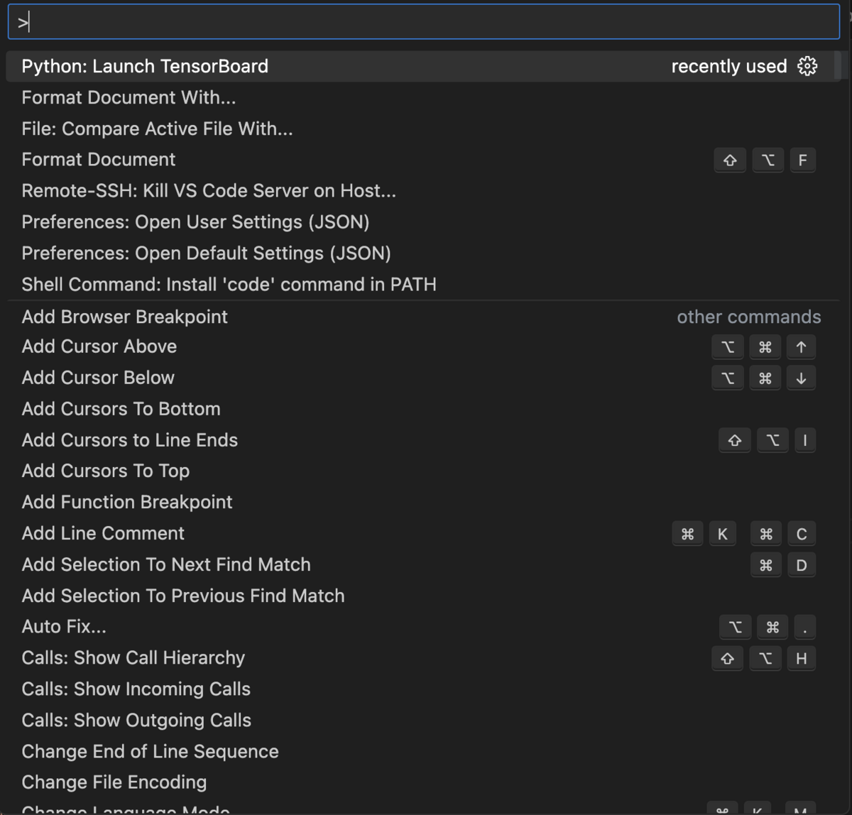
ここでは一番上に出てきている"Python: Launch TensorBoard"をクリックすると学習のパラメータや結果を保存しているディレクトリを指定することができます。

このリポジトリで作成したコードでは"logs/fit"がlogを保存するディレクトリになっているので、Select another folderをクリックした後、該当のパスを指定します。
Tensorboardでは学習の様子やモデルの構造を可視化・比較することができます。


分散共分散行列で定義された楕円体の断面算出
ある生物の神経細胞画像データを機械学習解析で使える形として抽出する。
アノテーションのデータがMATLABで解析されたファイルで与えられていた。
github.com
figshare.com
.matファイルから辞書データとして抜き出したところ、細胞の形が中心の座標と三次元の分散共分散行列で表されていた。
# 例
    # 中心座標
    center = [50, 50, 0]

    # 分散共分散行列
    # [x_var, xy_covar, zx_covar],
    # [xy_covar, y_var, yz_covar],
    # [zx_covar, yz_covar, z_var],

    cov_matrix = np.array(
        [
            [37.67218941864915, 9.97966493551884, 2.1263842045250754],
            [9.97966493551884, 14.353317888367672, 5.0364599497266935],
            [2.1263842045250754, 5.0364599497266935, 15.805485755173178],
        ]
    )
描画するとこんな感じ。
def show_ellipsoid(center, cov_matrix):
    # 固有値と固有ベクトルを計算
    eigenvalues, eigenvectors = np.linalg.eig(cov_matrix)

    # 楕円体を描画するためのパラメータ
    u = np.linspace(0, 2 * np.pi, 100)
    v = np.linspace(0, np.pi, 100)
    x = np.outer(np.cos(u), np.sin(v))
    y = np.outer(np.sin(u), np.sin(v))
    z = np.outer(np.ones(np.size(u)), np.cos(v))

    # 固有値に応じて楕円体を変形
    for i in range(len(eigenvalues)):
        x = np.sqrt(eigenvalues[i]) * (eigenvectors[0, i] * x)
        y = np.sqrt(eigenvalues[i]) * (eigenvectors[1, i] * y)
        z = np.sqrt(eigenvalues[i]) * (eigenvectors[2, i] * z)

    # 中心座標を追加
    x += center[0]
    y += center[1]
    z += center[2]

    # 3Dプロットを作成
    fig = plt.figure()
    ax = fig.add_subplot(111, projection="3d")

    # 楕円体をプロット
    ax.plot_surface(x, y, z, color="b", alpha=0.2)

    # 中心座標をプロット
    ax.scatter(center[0], center[1], center[2], color="r", s=100)

    # 軸ラベルの設定
    ax.set_xlabel("X")
    ax.set_ylabel("Y")
    ax.set_zlabel("Z")

    # グラフの表示
    plt.show()

顕微鏡で撮影された画像では上記のような楕円体の細胞が任意のzでスライスした楕円として観察される。
ChatGPTに助けてもらって関数を実装した。
def get_ellipse_intersection(center, cov_matrix, z):
    # 平面との交点で分散共分散行列を更新
    shifted_cov_matrix = cov_matrix.copy()
    shifted_cov_matrix[:2, :2] -= (z - center[2]) ** 2 * np.linalg.inv(
        cov_matrix[:2, :2]
    )

    # 2次元の分散共分散行列を抽出
    cov_2d = shifted_cov_matrix[:2, :2]

    # 固有値と固有ベクトルを計算
    eigenvalues, eigenvectors = np.linalg.eig(cov_2d)

    # 楕円のパラメータを計算
    semi_major_axis = np.sqrt(eigenvalues[0])
    semi_minor_axis = np.sqrt(eigenvalues[1])
    angle = np.arctan2(eigenvectors[1, 0], eigenvectors[0, 0])

    return semi_major_axis, semi_minor_axis, angle


def add_ellipse(canvas, x, y, semi_major_axis, semi_minor_axis, angle):
    center = (int(x), int(y))  # 中心座標を整数に変換
    axes = (int(semi_major_axis), int(semi_minor_axis))  # 軸の長さを整数に変換
    angle_degrees = int(np.degrees(angle))  # 角度を度数法に変換
    cv2.ellipse(
        canvas,
        center,
        axes,
        angle_degrees,
        0,
        360,
        255,
        thickness=-1,
    )
結果


多分あってるはず...
コードの全体図は以下の通りです。
import numpy as np
import matplotlib.pyplot as plt
import cv2
import math
import os


def show_ellipsoid(center, cov_matrix):
    # 固有値と固有ベクトルを計算
    eigenvalues, eigenvectors = np.linalg.eig(cov_matrix)

    # 楕円体を描画するためのパラメータ
    u = np.linspace(0, 2 * np.pi, 100)
    v = np.linspace(0, np.pi, 100)
    x = np.outer(np.cos(u), np.sin(v))
    y = np.outer(np.sin(u), np.sin(v))
    z = np.outer(np.ones(np.size(u)), np.cos(v))

    # 固有値に応じて楕円体を変形
    for i in range(len(eigenvalues)):
        x = np.sqrt(eigenvalues[i]) * (eigenvectors[0, i] * x)
        y = np.sqrt(eigenvalues[i]) * (eigenvectors[1, i] * y)
        z = np.sqrt(eigenvalues[i]) * (eigenvectors[2, i] * z)

    # 中心座標を追加
    x += center[0]
    y += center[1]
    z += center[2]

    # 3Dプロットを作成
    fig = plt.figure()
    ax = fig.add_subplot(111, projection="3d")

    # 楕円体をプロット
    ax.plot_surface(x, y, z, color="b", alpha=0.2)

    # 中心座標をプロット
    ax.scatter(center[0], center[1], center[2], color="r", s=100)

    # 軸ラベルの設定
    ax.set_xlabel("X")
    ax.set_ylabel("Y")
    ax.set_zlabel("Z")

    # グラフの表示
    plt.show()


def get_ellipse_intersection(center, cov_matrix, z):
    # 平面との交点で分散共分散行列を更新
    shifted_cov_matrix = cov_matrix.copy()
    shifted_cov_matrix[:2, :2] -= (z - center[2]) ** 2 * np.linalg.inv(
        cov_matrix[:2, :2]
    )

    # 2次元の分散共分散行列を抽出
    cov_2d = shifted_cov_matrix[:2, :2]

    # 固有値と固有ベクトルを計算
    eigenvalues, eigenvectors = np.linalg.eig(cov_2d)

    # 楕円のパラメータを計算
    semi_major_axis = np.sqrt(eigenvalues[0])
    semi_minor_axis = np.sqrt(eigenvalues[1])
    angle = np.arctan2(eigenvectors[1, 0], eigenvectors[0, 0])

    return semi_major_axis, semi_minor_axis, angle


def add_ellipse(canvas, x, y, semi_major_axis, semi_minor_axis, angle):
    center = (int(x), int(y))  # 中心座標を整数に変換
    axes = (int(semi_major_axis), int(semi_minor_axis))  # 軸の長さを整数に変換
    angle_degrees = int(np.degrees(angle))  # 角度を度数法に変換
    cv2.ellipse(
        canvas,
        center,
        axes,
        angle_degrees,
        0,
        360,
        255,
        thickness=-1,
    )


if __name__ == "__main__":
    os.makedirs("test_figs", exist_ok=True)
    os.makedirs("test_imgs", exist_ok=True)

    # 中心座標
    center = [50, 50, 0]

    # 分散共分散行列

    # [x_var, xy_covar, zx_covar],
    # [xy_covar, y_var, yz_covar],
    # [zx_covar, yz_covar, z_var],

    cov_matrix = np.array(
        [
            [37.67218941864915, 9.97966493551884, 2.1263842045250754],
            [9.97966493551884, 14.353317888367672, 5.0364599497266935],
            [2.1263842045250754, 5.0364599497266935, 15.805485755173178],
        ]
    )

    show_ellipsoid(center, cov_matrix)

    # 任意のz座標で交わる断面の楕円を求める
    for i, z in enumerate(range(-15, 15)):
        semi_major_axis, semi_minor_axis, angle = get_ellipse_intersection(
            center, cov_matrix, z
        )
        # 楕円を描画
        theta = np.linspace(0, 2 * np.pi, 100)
        x = semi_major_axis * np.cos(theta)
        y = semi_minor_axis * np.sin(theta)
        x_rotated = x * np.cos(angle) - y * np.sin(angle)
        y_rotated = x * np.sin(angle) + y * np.cos(angle)

        plt.figure(figsize=(5, 5))
        plt.plot(x_rotated + center[0], y_rotated + center[1])
        plt.xlim(40, 60)
        plt.ylim(40, 60)
        plt.xlabel("X")
        plt.ylabel("Y")
        plt.title(f"Ellipse Intersection with z={z} Plane")
        plt.grid(True)
        plt.savefig(f"test_figs/{i:03}.png")
        plt.close()

        xy_canvas = np.zeros((100, 100), dtype="uint8")
        if (
            math.isnan(semi_major_axis) == False
            and math.isnan(semi_minor_axis) == False
        ):
            add_ellipse(
                xy_canvas, center[0], center[1], semi_major_axis, semi_minor_axis, angle
            )

        cv2.imwrite(f"test_imgs/{i:03}.png", xy_canvas)
PyTorch-Lightningのチュートリアルがちゃんと動かない
チュートリアルが動かない?意味ねえじゃん
結論から言うと最初の実行セルを
!pip install segmentation-models-pytorch
# !pip install pytorch-lightning==1.5.4
!pip install pytorch-lightning==1.9.5
と変更すればよかった。
以下のチュートリアルをgoogle colabで動かそうとした。
セグメンテーションタスクのサンプルとして以下のサイトで紹介されていた。
!pip install segmentation-models-pytorch
!pip install pytorch-lightning==1.5.4

import os
import torch
import matplotlib.pyplot as plt
import pytorch_lightning as pl
import segmentation_models_pytorch as smp

from pprint import pprint
from torch.utils.data import DataLoader

---------------------------------------------------------------------------
ModuleNotFoundError                       Traceback (most recent call last)
<ipython-input-2-495d7f80e44f> in <cell line: 4>()
      2 import torch
      3 import matplotlib.pyplot as plt
----> 4 import pytorch_lightning as pl
      5 import segmentation_models_pytorch as smp
      6

4 frames
/usr/local/lib/python3.10/dist-packages/pytorch_lightning/utilities/apply_func.py in <module>
     28 if _TORCHTEXT_AVAILABLE:
     29     if _compare_version("torchtext", operator.ge, "0.9.0"):
---> 30         from torchtext.legacy.data import Batch
     31     else:
     32         from torchtext.data import Batch

ModuleNotFoundError: No module named 'torchtext.legacy'
importでこけるんかい
ひとまずtorchtextを追加でインストールしてみる。
!pip install segmentation-models-pytorch
!pip install pytorch-lightning==1.5.4
!pip install torchtext
同じエラーで進まず。
----> 4 import pytorch_lightning as pl
ModuleNotFoundError: No module named 'torchtext.legacy'
ググって見つけた情報を順番に試す。
!pip install segmentation-models-pytorch
!pip install pytorch-lightning==1.5.4
!pip install torchtext==0.10.0

ERROR: Could not find a version that satisfies the requirement torchtext==0.10.0 (from versions: 0.1.1, 0.2.0, 0.2.1, 0.2.3, 0.3.1, 0.4.0, 0.5.0, 0.6.0, 0.12.0, 0.13.0, 0.13.1, 0.14.0, 0.14.1, 0.15.1, 0.15.2)
ERROR: No matching distribution found for torchtext==0.10.0
💢
!pip install segmentation-models-pytorch
!pip install pytorch-lightning==1.5.4
!pip install torchtext==0.14.0

- 中略 -

ERROR: pip's dependency resolver does not currently take into account all the packages that are installed. This behaviour is the source of the following dependency conflicts.
torchaudio 2.0.2+cu118 requires torch==2.0.1, but you have torch 1.13.0 which is incompatible.
torchdata 0.6.1 requires torch==2.0.1, but you have torch 1.13.0 which is incompatible.
torchvision 0.15.2+cu118 requires torch==2.0.1, but you have torch 1.13.0 which is incompatible.
Successfully installed torch-1.13.0 torchtext-0.14.0
エラーが出ているが0.14.0がインストールできているようなので続行してみる。
---------------------------------------------------------------------------
ImportError                               Traceback (most recent call last)
<ipython-input-2-495d7f80e44f> in <cell line: 4>()
      2 import torch
      3 import matplotlib.pyplot as plt
----> 4 import pytorch_lightning as pl
      5 import segmentation_models_pytorch as smp
      6

4 frames
/usr/local/lib/python3.10/dist-packages/pytorch_lightning/utilities/apply_func.py in <module>
     30         from torchtext.legacy.data import Batch
     31     else:
---> 32         from torchtext.data import Batch
     33 else:
     34     Batch = type(None)

ImportError: cannot import name 'Batch' from 'torchtext.data' (/usr/local/lib/python3.10/dist-packages/torchtext/data/__init__.py)
うーん、深みにハマってしまっている気がする。
一旦初期状態に戻してみる。
pytorch-lightningのversionを変更してみた。
!pip install segmentation-models-pytorch
# !pip install pytorch-lightning==1.5.4
!pip install pytorch-lightning==1.9.5
これでimportのエラーは出なくなった。
この後のtrainningも動いたのでよしとする。
ちなみに
バージョンを指定せずにinstallすると...
!pip install segmentation-models-pytorch
# !pip install pytorch-lightning==1.5.4
!pip install pytorch-lightning
importではエラーは出ないが
trainer = pl.Trainer(
    gpus=1,
    max_epochs=5,
)

trainer.fit(
    model,
    train_dataloaders=train_dataloader,
    val_dataloaders=valid_dataloader,
)
のセルを実行すると
---------------------------------------------------------------------------
TypeError                                 Traceback (most recent call last)
<ipython-input-9-f1c61f5ae996> in <cell line: 1>()
----> 1 trainer = pl.Trainer(
      2     gpus=1,
      3     max_epochs=5,
      4 )
      5

/usr/local/lib/python3.10/dist-packages/pytorch_lightning/utilities/argparse.py in insert_env_defaults(self, *args, **kwargs)
     67
     68         # all args were already moved to kwargs
---> 69         return fn(self, **kwargs)
     70
     71     return cast(_T, insert_env_defaults)

TypeError: Trainer.__init__() got an unexpected keyword argument 'gpus'
pytorch-lightning v2から仕様が変わっているらしい。
このサイトに従って
trainer = pl.Trainer(max_epochs=5,accelerator="auto")

trainer.fit(
    model,
    train_dataloaders=train_dataloader,
    val_dataloaders=valid_dataloader,
)

INFO:pytorch_lightning.utilities.rank_zero:GPU available: True (cuda), used: True
INFO:pytorch_lightning.utilities.rank_zero:TPU available: False, using: 0 TPU cores
INFO:pytorch_lightning.utilities.rank_zero:IPU available: False, using: 0 IPUs
INFO:pytorch_lightning.utilities.rank_zero:HPU available: False, using: 0 HPUs
gpuは認識できたっぽいが
---------------------------------------------------------------------------
NotImplementedError                       Traceback (most recent call last)
<ipython-input-10-dbbdb5087c44> in <cell line: 3>()
      1 trainer = pl.Trainer(max_epochs=5,accelerator="auto")
      2
----> 3 trainer.fit(
      4     model,
      5     train_dataloaders=train_dataloader,

5 frames
/usr/local/lib/python3.10/dist-packages/pytorch_lightning/trainer/configuration_validator.py in __verify_train_val_loop_configuration(trainer, model)
     77     # check legacy hooks are not present
     78     if callable(getattr(model, "training_epoch_end", None)):
---> 79         raise NotImplementedError(
     80             f"Support for `training_epoch_end` has been removed in v2.0.0. `{type(model).__name__}` implements this"
     81             " method. You can use the `on_train_epoch_end` hook instead. To access outputs, save them in-memory as"

NotImplementedError: Support for `training_epoch_end` has been removed in v2.0.0. `PetModel` implements this method. You can use the `on_train_epoch_end` hook instead. To access outputs, save them in-memory as instance attributes. You can find migration examples in https://github.com/Lightning-AI/lightning/pull/16520.
と言うことでまた関数名や仕様が変わっておりうまくいかない。
同じv1系の最新バージョンを使うことでなんとか動かした。
原理的にはv2系でも動かせるはずだが今日はここまで。
matplotlibで統計・系統誤差付きの図を作る(python)
かなり久々の更新。
matplotlibとpythonで統計誤差、系統誤差を描写する簡単なスクリプト
こんな感じの図が書けます(今回は横軸Event No、縦軸が測定値や誤差など)
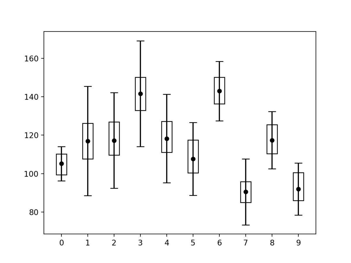
Eventごとに統計誤差、系統誤差が異なる場合の絵ですね。
同じ研究対象に対するいくつかの実験結果をまとめる際などに使われがちです。
他にいい方法をご存知の方がいましたらご教授ください。
import numpy as np
import matplotlib.pyplot as plt
import matplotlib.patches as patches
import random

if __name__ == '__main__':

    mean_values = np.random.normal(100, 20, 10)  # 平均100、標準偏差20、event数10
    stat_errors = np.random.normal(20, 5, 10)  # 測定誤差の平均が20、ばらつきが5

    # 正負に非対称な誤差がつくことを想定
    syst_errors = []
    for i in range(len(mean_values)):
        syst_high = random.uniform(5, 10)
        syst_low = random.uniform(5, 10)
        syst_errors.append([syst_high, syst_low])


    fig, ax = plt.subplots()

    #Eventに番号付け
    events = list(range(len(mean_values)))

    # 誤差棒ありのplot
    plt.errorbar(events, mean_values, stat_errors, capsize=5, fmt='o', markersize=5, ecolor='black', markeredgecolor="black", color='k')

    # 各Eventで系統誤差を示すboxを描写
    event_counter = 0
    for meam, syst in zip(mean_values, syst_errors):
        r = patches.Rectangle(xy=(event_counter-0.2, meam-syst[1]), width=0.4, height=sum(syst), ec='k', fill=False)
        ax.add_patch(r)
        event_counter += 1

    ax.set_xticks(range(10))
    plt.show()
ポイントはmatplotlib.patchesです。
note.nkmk.me
matplotlibにはeventplotという関数があって名前がそれっぽいと思ったのですが全然違いました…
自前のMask画像からCOCO format jsonを作成
手作業でAnnotationなんてやってられるか!!!
ということで、画像処理でcoco formatのjsonを作るscriptを書きました。
簡易的なのでぜひ改造して使ってください。
ただしMask情報が二値化画像で取得できている前提です。
そもそも二値化できるなら物体検出いらないというツッコミはさておき…

Mask R-CNN
機械学習において最も注目されている分野の一つが物体検出です。
自動運転や監視カメラなど、画像・映像情報から注目したい物体を抽出する技術で直感的かつ応用の幅が広い技術です。
その中でも有名かつ、開発が盛んなのがMask R-CNNと呼ばれる手法です。
論文はこちら
https://arxiv.org/abs/1703.06870
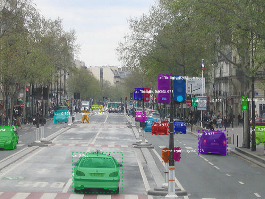
こんな感じで画像中から物体を検出し、それぞれがなんであるかを判断しています。
開発の歴史はこちらの記事によくまとまっています。
qiita.com
非常に優れた手法ですが、最初からこんな結果が得られるわけではなく、学習が必要です。
機械学習modelは正解の情報を持っている教師データを元に、最適な内部の重みを決定しています。
(機械学習について詳しく知りたい人はこちら。私も超初心者で勉強中です。)
ゼロから作るDeep Learning ―Pythonで学ぶディープラーニングの理論と実装 斎藤 康毅
https://www.amazon.co.jp/dp/4873117585/ref=cm_sw_r_tw_dp_x_42Y3Fb1GA2SF8
機械学習スタートアップシリーズ これならわかる深層学習入門 (KS情報科学専門書) 瀧 雅人
https://www.amazon.co.jp/dp/4061538284/ref=cm_sw_r_tw_dp_x_e4Y3Fb8MTHZK4
先程の画像のように様々な物体を精度よく検出するためには大量の画像とそれぞれに正解の情報が必要です。
そこでデータセットとして学習および性能検証に用いられるベンチマークがCOCO datasetと呼ばれる巨大なdatasetです。
COCO dataset
"Common Objects in Context" 略してCOCO。
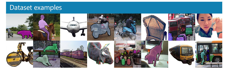
下の画像で示すように様々な画像と物体、それぞれが何であるか記述された正解情報をもっています。
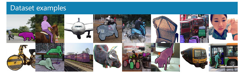
正解情報を持つjsonはこんな感じ。
https://docs.trainingdata.io/v1.0/Export%20Format/COCO/
{
  "info" : info,
  "images" : [image],
  "annotations" : [annotation],
  "licenses" : [license],
}

info: {
  "year" : int,
  "version" : str,
  "description" : str,
  "contributor" : str,
  "url" : str,
  "date_created" : datetime,
}

image: {
  "id" : int,
  "width" : int,
  "height" : int,
  "file_name" : str,
  "license" : int,
  "flickr_url" : str,
  "coco_url" : str,
  "date_captured" : datetime,
}

license: {
  "id" : int,
  "name" : str,
  "url" : str,
}
このデータセットが基準となるformatをもっていることによって異なるmodelでも性能が比較できるようになっています。
またjsonのformatを揃えることで様々なデータを入れ替えても同じプログラム上で動くようになっています。
しかし、実際自分で使う際には専用の学習データを使って目的に特化したmodelを作成したいものです。
そのためには画像の中の正解情報を取得するAnnotation作業が必須になります。
Annotation作業
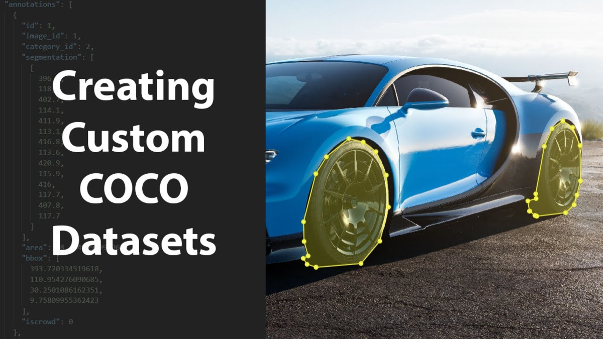
めちゃくちゃめんどくさそう…
数枚ならまだしも学習データは数千枚になる場合が多いので手作業でぽちぽちしていると寿命が尽きてしまいます。
複雑な物体に対しては人間の手が必要ですが、簡易的な画像に対しては楽ができるはずです。
画像処理によるcoco format jsonの生成
用意した画像はこちらからダウンロードしました。
https://www.cis.upenn.edu/~jshi/ped_html/PennFudanPed.zip
簡単のため人がひとりしか写っていない画像だけをえらんでいます。
もちろん、複数の場合でもちょっとした改造を加えれば処理が可能です。
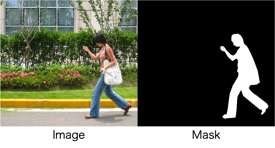
Imageとmaskは同じ名前にしています。
  ┠ images
  ┃  ┠ 00001.png
  ┃  ┠ 00002.png
  ┃  ┠ 00003.png
  ┃  ┠ 以下略
  ┠ masks
  ┃  ┠ 00001.png
  ┃  ┠ 00002.png
  ┃  ┠ 00003.png
  ┃  ┠ 以下略
import json
import collections as cl
import numpy as np
import matplotlib.pyplot as plt
from scipy import ndimage
from skimage import measure
from skimage.segmentation import clear_border
from skimage.filters import threshold_otsu
import cv2
import glob
import sys
import os

### https://qiita.com/harmegiddo/items/da131ae5bcddbbbde41f

def info():
    tmp = cl.OrderedDict()
    tmp["description"] = "Test"
    tmp["url"] = "https://test"
    tmp["version"] = "0.01"
    tmp["year"] = 2020
    tmp["contributor"] = "salt22g"
    tmp["data_created"] = "2020/12/20"
    return tmp

def licenses():
    tmp = cl.OrderedDict()
    tmp["id"] = 1
    tmp["url"] = "dummy_words"
    tmp["name"] = "salt22g"
    return tmp

def images(mask_path):
    tmps = []
    files = glob.glob(mask_path + "/*.png")
    files.sort()

    for i, file in enumerate(files):
        img = cv2.imread(file, 0)
        height, width = img.shape[:3]

        tmp = cl.OrderedDict()
        tmp["license"] = 1
        tmp["id"] = i
        tmp["file_name"] = os.path.basename(file)
        tmp["width"] = width
        tmp["height"] = height
        tmp["date_captured"] = ""
        tmp["coco_url"] = "dummy_words"
        tmp["flickr_url"] = "dummy_words"
        tmps.append(tmp)
    return tmps


def annotations(mask_path):
    tmps = []

    files = glob.glob(mask_path + "/*.png")
    files.sort()

    for i, file in enumerate(files):
        img = cv2.imread(file, 0)
        tmp = cl.OrderedDict()
        contours = measure.find_contours(img, 0.5)
        segmentation_list = []

        for contour in contours:
            for a in contour:
                segmentation_list.append(a[0])
                segmentation_list.append(a[1])


        mask = np.array(img)
        obj_ids = np.unique(mask)
        obj_ids = obj_ids[1:]
        masks = mask == obj_ids[:, None, None]
        num_objs = len(obj_ids)
        boxes = []

        for j in range(num_objs):
            pos = np.where(masks[j])
            xmin = np.min(pos[1])
            xmax = np.max(pos[1])
            ymin = np.min(pos[0])
            ymax = np.max(pos[0])
            boxes.append([xmin, ymin, xmax, ymax])

        tmp_segmentation = cl.OrderedDict()

        tmp["segmentation"] = [segmentation_list]
        tmp["id"] = str(i)
        tmp["image_id"] = i
        tmp["category_id"] = 1
        tmp["area"] = float(boxes[0][3] - boxes[0][1]) * float(boxes[0][2] - boxes[0][0])
        tmp["iscrowd"] = 0
        tmp["bbox"] =  [float(boxes[0][0]), float(boxes[0][1]), float(boxes[0][3] - boxes[0][1]), float(boxes[0][2] - boxes[0][0])]
        tmps.append(tmp)
    return tmps

def categories():
    tmps = []
    sup = ["person"]
    cat = ["person"]
    for i in range(len(sup)):
        tmp = cl.OrderedDict()
        tmp["id"] = i+1
        tmp["name"] = cat[i]
        tmp["supercategory"] = sup[i]
        tmps.append(tmp)
    return tmps

def main(mask_path, json_name):
    query_list = ["info", "licenses", "images", "annotations", "categories", "segment_info"]
    js = cl.OrderedDict()
    for i in range(len(query_list)):
        tmp = ""
        # Info
        if query_list[i] == "info":
            tmp = info()

        # licenses
        elif query_list[i] == "licenses":
            tmp = licenses()

        elif query_list[i] == "images":
            tmp = images(mask_path)

        elif query_list[i] == "annotations":
            tmp = annotations(mask_path)

        elif query_list[i] == "categories":
            tmp = categories()

        # save it
        js[query_list[i]] = tmp

    # write
    fw = open(json_name,'w')
    json.dump(js,fw,indent=2)

args = sys.argv
mask_path = args[1]
#mask_path =  ""
json_name = args[2]
#json_name = "person_sample.json"

if __name__=='__main__':
    main(mask_path, json_name)
こちらの記事を参考にさせていただきました。ありがとうございました
。
qiita.com
肝となるのはこの部分です。
contours = measure.find_contours(img, 0.5)
find_contoursは画像中の物体の輪郭のpix座標を取得してくれます。
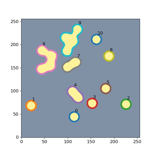
また、bboxについては
pos = np.where(masks[j])
この部分で取得したmask情報を持つpixの最大値最小値を使っています。
Mask R-CNNのdemo codeを参考にしています。
pytorch.org
取得したjson fileはこちら。
{
  "info": {
    "description": "Test",
    "url": "https://test",
    "version": "0.01",
    "year": 2020,
    "contributor": "salt22g",
    "data_created": "2020/12/20"
  },
  "licenses": {
    "id": 1,
    "url": "dummy_words",
    "name": "salt22g"
  },
  "images": [
    {
      "license": 1,
      "id": 0,
      "file_name": "FudanPed00011.png",
      "width": 459,
      "height": 420,
      "date_captured": "",
      "coco_url": "dummy_words",
      "flickr_url": "dummy_words"

   #〜中略〜#

  ],
    "annotations": [
      {
        "segmentation": [
          [
            48.0,
            129.00229357798165,
            47.96153846153846,
            129.0,
            48.0,
            128.9878048780488,
            48.016129032258064,
            129.0,
            48.0,

   #〜中略〜#

      "id": "0",
      "image_id": 0,
      "category_id": 1,
      "area": 62868.0,
      "iscrowd": 0,
      "bbox": [
        36.0,
        55.0,
        156.0,
        403.0
      ]
    },

   #〜中略〜#

  ],
  "categories": [
    {
      "id": 1,
      "name": "person",
      "supercategory": "person"
    }
  ],
  "segment_info": ""
}
元の画像とこのjson fileがあればほとんどのCOCOを基準に開発されている物体検出が動くはず。
ではまた。